The ecosystem of trading in financial markets hosts a variety of strategies that, depending on the inefficiency that they try to exploit, are amenable of being included in some of the primary categories. One of these categories is trend following, and one of the best known core strategies in this category is moving average crossover. These strategies include two (or more) moving averages configured with different periods, in such a way that crossovers where the fast (i.e. lower period) moving average crosses over the slow (i.e. higher period) moving average provide buying signals, whereas crossovers where the fast moving average crosses under the slow one provide selling signals. In this study, the slow moving average is a simple moving average (SMA), and the fast one is an exponential moving average (EMA), but the same methodology may apply to any other types of moving averages.
Stock indices exhibit trending behaviours in any timeframe, and a trend following strategy tries to capture those trending movements as much as possible. The asset selected for this study is the Spanish IBEX-35 index, in the timeframe M1, which provides a large number of trading signals making it possible to reach statistical significance.
Why predict crossovers?
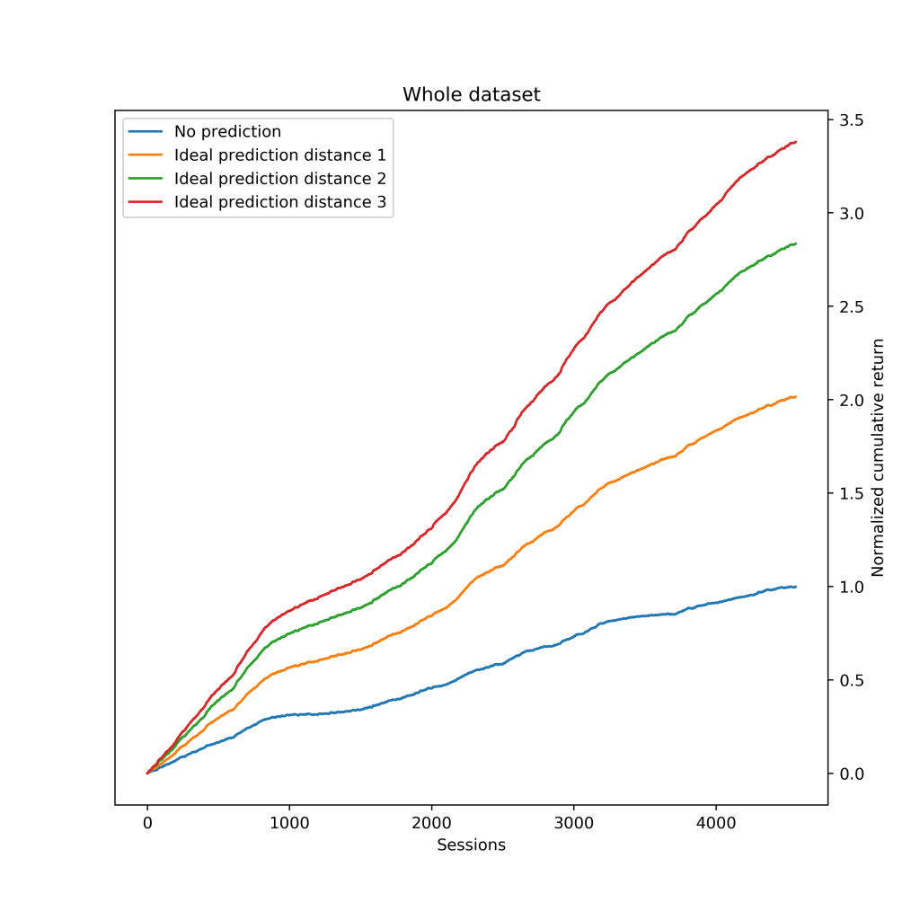
Crossovers mostly occur once a trending movement has unfolded a not negligible stretch. Thus, it seems expectable that being able to get the trading signal before the crossover actually occurs would capture, on average, a greater portion of the movement, therefore increasing the strategy expectation. This was confirmed by a simulation which yielded the following results: The blue line depicts the baseline, which is the gross cumulative return of the crossover strategy over the whole data sample. If we were able to correctly predict 100% of the crossovers just one sample before it occurs, the expectation of the strategy increases an astonishing 100% (orange line). Earlier predictions (green and red lines) yield higher expectation, but this also makes the prediction much harder. All the results presented hereinafter are based on predictions at distance 1.
Feature selection
The proposal is to predict crossovers based on the previous behaviour of the moving averages. In this study, moving averages, of periods ![]() and
and ![]() at the sample
at the sample ![]() , are defined based solely on the closing price as follows:
, are defined based solely on the closing price as follows:
![]()

The number of previous moving average values becomes a hyperparameter of the estimator. We call it delay (![]() ). Notice that it actually turns out in predicting whether the price of the next sample will be higher or lower than a threshold (i.e. the price that makes
). Notice that it actually turns out in predicting whether the price of the next sample will be higher or lower than a threshold (i.e. the price that makes ![]() ). Given the previous definitions, and solving for
). Given the previous definitions, and solving for ![]() , this threshold is:
, this threshold is:
![]()
Data preprocessing
Raw data to work with are the historical quotes of the asset analyzed. Each sample includes the following fields:
![]()
The first step is computing the ![]() and
and ![]() for each sample from the raw data. Then, it is key to extract relative price movements from the absolute values of computed moving averages in order to properly reflect price behaviour. That is:
for each sample from the raw data. Then, it is key to extract relative price movements from the absolute values of computed moving averages in order to properly reflect price behaviour. That is:
![]() where
where ![]()
Since we want to reveal the moving average behaviour with respect to each other, each single value is first scaled within the range of each estimator sample, and then feature reduction is applied by substracting each pair:
![]()
This transformation also ensures every single estimator input is within the range ![]() .
.
Finally, because this problem suffers from class imbalance (just 5.65% of the total samples are crossovers, and they are the key class), the estimators build biased models. Given the huge dataset available, larger than 2.2M samples, among the repertory of techniques to deal with this issue, undersampling was applied by removing ∼90% randomly selected non-crossovers samples.
Prediction model
Two different estimators were evaluated: multilayer perceptron (MLP) and support vector machine (SVM) with the following setup:
- Binary classificator
- Prediction distance: 1
- Delay: 5
- Training period: [00/02, 12/06]: 239,910 samples (70%)
- Test period: [12/07, 17/12]: 101,961 samples (30%)
Due to the nature of this problem, hits are defined as those predicted crossovers that actually were, and misses as those predicted crossovers that actually were not. That is, we neither include non-crossovers correctly predicted as hits nor crossovers that were not predicted as misses. Both estimators, MLP and SVM, performed really similarly, reaching hit rates of [0.88, 0.89] and almost equalling the number of actual crossovers in their inferences.
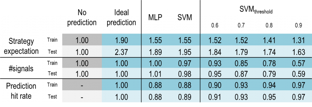
Hit rate is a valuable metric, but, in order to evaluate the prediction model, it is essential to verify how predictions translate into expectation. The following chart shows the cumulative return along the training period normalized to the maximum reached in the baseline case (no prediction). An ideal prediction in this subset would increase the cumulative return by a factor of 1.90. Both estimators, MLP and SVM, outperform the baseline by 1.55.
 In the test subset, an ideal prediction would increase cumulative return by 2.37, whereas MLP does by 1.89, and SVM by 1.95. In summary, the prediction model is able to perform ∼61% the oracle in the training subset and ∼82% in the test subset.
Beyond accuracy
The results presented so far were obtained with the classifier threshold set to 0.5. Keeping in mind that the objetive is to enhance a trading strategy, does it make sense to move that threshold? We can face different scenarios when aiming to improve such strategy depending on how our baseline strategy performs. If it is already a winner, then we should explore tradeoffs between expectation and volume of signals generated. On the contrary, if it is not even able to overcome the operational costs, increasing expectation becomes mandatory.
According to the results, the prediction model still has room for improvement as it performs ∼30% under the oracle. It seems expectable that selecting a more restrictive classifier threshold would yield higher accuracy, and therefore higher expectation, at the expense of decreasing the trading signals.
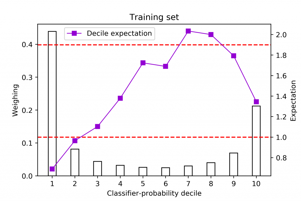
This chart reveals that distribution both for MLP and SVM estimators. The ocurrence ratio is calculated for each class given a threshold of 0.5. Most non-crossover predictions are gathered on the first decile while most crossovers are on the last decile. Hence, no heavy changes are expected unless changes on the threshold exclude the first and/or the last decile. We can also see how similar both estimators are, so for the rest of the analysis only SVM is explored.
A first approach where higher expectation is desired sets the classifier threshold beyond 0.5. The following table summarizes all the scenarios focusing on the three key metrics. Expectation and #signals are normalized to a baseline case where no predictions are made, whereas the baseline for prediction hit rate is the ideal prediction, as making no predictions does not apply.
This study reports interesting insights. On one hand, the metrics #signals and hit rate behave as expected: the higher the threshold the higher the hit rate at the expense of losing signals. On the other hand, expectation does not match hit rate trend as it worsens as the threshold increases. Let us find out how hit rate and expectation correlate over the whole probability space.
These charts plot three components. First, the lower and upper dashed red lines point out the expectation of the baseline (making no predictions), and the expectation of the oracle (ideal prediction), respectively. Second, bars measure the weighing of each decile over the whole probability space. And third, the violet squares illustrate the expectation for each classifier-probability decile. Correlation between the hit rate and expectation observed in the first half of deciles, no longer remains in the second half, specially in the last decile, which also turns out to be the one that gathers the greatest number of crossover predictions.
Recalling what we stated at the beginning of this section, a look at these analysis reveals different opportunities to optimally set our estimators. For instance, strategies that are strong enough at any point above the lower red line, may benefit from setting a lower classifier threshold, as more profitable signals would be provided, turning out, more likely, in a longer time-in-market. On the contrary, those strategies demanding more expectation, may consider excluding predictions coming from the last decile, as long as losing its remarkable volume of signals is acceptable.


Bien fran!!!