The first article of the serie Trading misconceptions analyzed a technique very popular within the trader’s community. The technique discussed in this article is even more popular, in fact, it is considered as one of the mainstays of a successful system. If were asked to summarize this technique in a single sentence, I would say: “Always keep a bullet in the chamber”. It is especially found when trades do not progress as expected, adding more positions as the price moves against our interests. In my opinion, the three key factors responsible for applying this technique are:
- Lack of stop loss
- Lack of a well defined signals
- Vague knowledge about money management
At least one of these factors, if not all, are present when a trader defends this technique. I could also point out another factor which has to do with the pyschological aspect (as many things in trading!), but it actually is a consequence of the first one: the reluctance to accept losses. The trader’s mind joins new positions with the previous losser opened trades, in such a way that average price is closer to the current price. If the price later reaches this average, they feel comfortable closing all of them because they think of them as a single trade, and therefore they are not lossing.
Strategy simulation
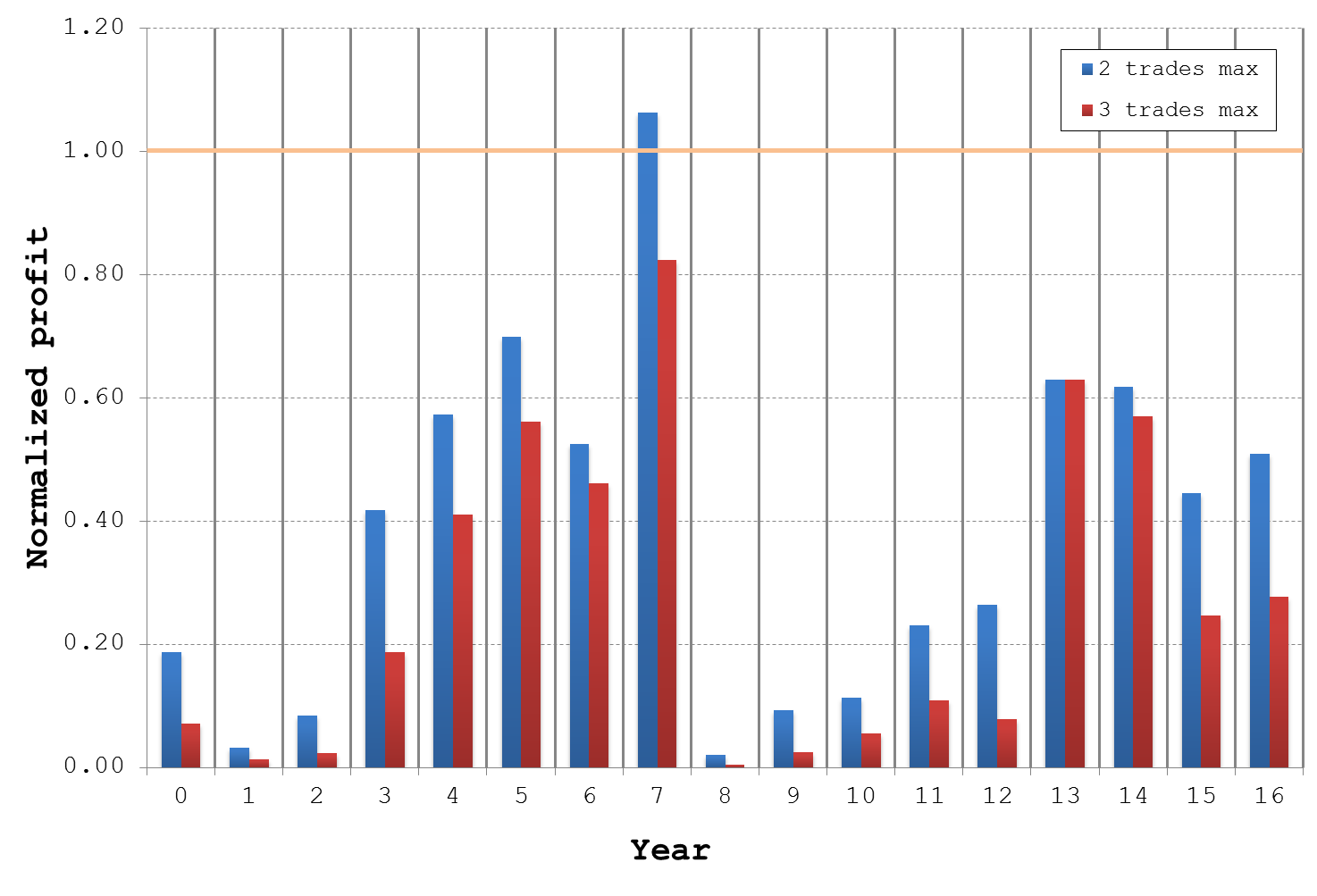
The metric par excellence when presenting the performance of a system is cumulative profitability over the sampled data. Indeed, it should be the starting point when analyzing the validity of a strategy, but we must be careful of what conclusions we draw from it. Have a look at the graph below this lines. Which one would you choose? Probably the most repeated answer would be: “the blue one”. It reaches the largest cumulative profitabilty by far, and the curve shape looks like the other alternatives (i.e. similar variance), so it is tempting to choose it if we do not know what this metric really means and which implications may have some others factors regarding the actual performance. Let me give you some additional information…

The underlying strategy is the same in the three alternatives: Same signals, same stop loss and the take profit, and same time frame. What is the difference then? Due to the fact that trades in this strategy are independent events (i.e. neither a short trade closes a previous long nor viceversa, and new trades do not modify any previous trade parameter), multiple trades coexist (3.1±3.8). All three alternatives graphed have limited the number of coexisting trades. This restriction has the effect of discarding trades, whose outcome is known to be positive if the sample is big enough. Hence, the higher the restriction the lower the cumulative profitability.
Now the question is: how does this metric translates into the actual performance? Here is where reciprocal interactions between strategy and MM come into play.
System simulation
Once we have validated our strategy through the previous simulation, it is time to analyze its behaviour regarding the MM parameters. This step is as crucial as having a good strategy; a carefully adjusted MM can strongly improve its performance. I compared the actual profit of the same strategy on a yearly basis limiting the spreading degree. The results are normalized to the best choice, that is no spreading, so values under 1.0 are not desirable.
The MM analyzed has the following features:
- Maximum leverage: ∼6.0
- Exposure dynamically adjusted with a trade-by-trade granularity
- Profit cashout on a yearly basis
- Longs and shorts compensate for the net exposure
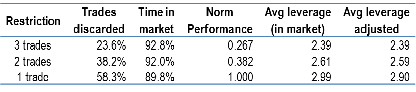
Look at the table underneath; just one degree of spreading – shooting and keeping one bullet on the chamber – reduces the average yearly profit by a 61.8% (does this ratio sound familiar to you?), and the more we spread trades out the more the profit is reduced. I’d like to highlight the rightmost column, which measures the effective leverage by weightening time in market, because it is the key metric which explains the results: The higher the spread degree the lower the effective leverage.
Dealing with big swings
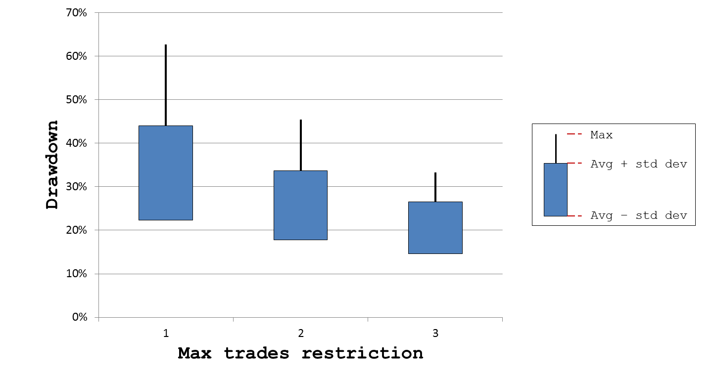
The analysis presented so far revealed the big opportunity cost of spreading out trades. However, it also has a remarkable effect on the account variance, to the extent of not being feasible for certain trader’s profiles. The chart shows how drawdowns distribution vary according to the maximum number of coexisting trades. The most profitable choice entails drawdowns of 33.2%±10.9% with a peak of 62.7%. Allowing up to two coexisting trades reduces the average size of swings by ∼23% (25.2%±10.9%; 62.7%). Finally, if we allow our system to mantain up to 3 coexisting trades, drawdowns are reduced by ∼38% (20.6%±5.9%; 33.3%).
Are all traders ready to bear such big swings? Obviously not. Drawdowns as large as 60% are incompatible with risk aversion threshold of many traders; they will likely end giving up using their systems when facing such variance. This underscores how critical is to carefully make this kind of calculations in order to know what can we expect, and therefore being able to distinguish what’s normal behaviour from what is not. For those traders who can not sleep peacefully with big swings I suggest to choose more stable setups at the expense of sacrificing performance.
bien fran!!